
Introduction
This article is just going to serve as a relatively brief and informal explanation of the little project I undertook over the past few weeks. This isn’t going to be any kind of tutorial, but I’ll make sure to drop a few links at the end if you are interested in getting started with Demoscene type stuff yourself!
Video
A Quick Bit of Background Material
Before I start going into detail with the techniques I used, I first need to emphasise exactly what is going on in the video and why I chose to do things like this! The techniques I am using are similar to those that you would find over on Shadertoy.com, and I would wholeheartedly recommend checking that website out if you have an interest in procedural graphics! Specifically, instead of rendering a bunch of polygons to the screen as is common in 3D graphics I am rendering a single quad that encompass the entire screen. This quad can be used as a canvas for the visuals! I then render onto this canvas per-pixel, entirely procedurally. This means that no models or textures were pre-made; everything is lovingly generated at runtime! Unfortunately, generating 60 frames per second in this fashion is expensive, but it can be achieved with fragment shaders on a not shit GPU!
If you are not familiar with fragment shaders or what they are exactly, I’ll give a quick explanation now. Without going into detail about their place in the OpenGL programmable graphics pipeline (words words…), the gist of fragment shaders is that each time a fragment shader is executed, a bunch of inputs are taken and the colour of one pixel is outputted. Typically, they will take inputs of a texture, per-fragment texture coordinates, texture resolution and a series of other useful and custom inputs to drive the rendering. Once inputs are taken, a bunch of processing ensues and the colour of the pixel is spat out at the end! Another thing to note is that all data you take in and process during a fragment shader’s execution is volatile and lost once the colour of the pixel is output, meaning there is no dependency on other instances of the shader’s execution. This makes it absolutely ripe for parallelisation and for use on GPU hardware. This is why they are so fast!
Example
#version 430

//Texture coordinates being passed into the fragment shader
//Both the x and y components are in the range 0 to 1
in vec2 uv;

//Main function; the entry point for the shader
void main()
{
  //RGB values are also defined in the range 0 to 1, so coordinates can be used as colour values
  vec3 color = vec3(uv.x, 1.0, uv.y);

  //Outputting the colour (with a forced alpha channel of 1)
  gl_FragColor = vec4(color, 1.0);
}
One problem that arises is that, while processing, the program has no idea of what the neighbouring pixels look like - this can partly be solved using a technique called multipass rendering, but I’ll get onto that later. You may also be wondering why I bother doing things in this way, rather than use polygons! The core idea behind Demoscene culture is to show off, but to also push hardware to its limits. Depending on the category, demosceners also try to render things that are impressive while also using as little storage as possible. Although I am not going the full mile with this demo (I didn’t really try and compress anything…) I wanted to adhere to two rules I set myself; no pre-made assets and no imported files besides the music. This aligns with the demos you see over on Shadertoy.com! Of course, I am excluding my logo from the introduction in this, but sssshhhh.
As one last note, I absolutely urge people reading this to check out some of the demos people have made in the past, a lot of which are available to view on Youtube! I guarantee you will have your mind blown! One of my personal favourites is Monolith by ASD, which is a real-time demo in under a compressed 256MB. For something more recent and quite frankly, absolutely ridiculous, there is also this incredible 4K demo (4 kilobytes! This webpage is bloody 38KB!) that came out this year at Revision; Absolute Territory (MAJOR EPILEPSY WARNING) by Prismbeings. I can only hope to get this good in the future!
How the Rendering Works
Now that everyone is on the same page when concerned with fragment shaders (or at least briefly how they work…), I can explain how you can use a fragment shader to produce a fully realised 3D scene. I’m going to reiterate that this is not a tutorial and merely a quick explanation of how I personally went about things to provide a little insight - if you want a detailed guide on how to do this yourself, please refer to the links at the bottom of the page!
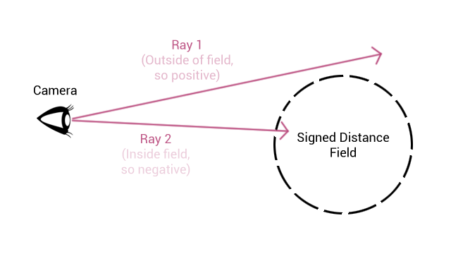
There are two key aspects in the rendering; the first is a technique called Ray Marching and the second is the use of Signed Distance Functions (in 3D graphics and certainly the Demoscene, these tend to be called Signed Distance Fields. I will refer to them as such from now on). If you’ve looked into 3D graphics previously, then you might have come across ray marching. Just in case, I’ll explain anyway: ray marching is a technique whereby from a point in space (usually the camera) a ray is “cast” out into the environment. This ray is then stepped, or marched, along incrementally until either an object is hit or a maximum threshold is breached. The technique integrates into 3D graphics nicely - for each pixel on the screen, a ray can be cast out and stepped along. If the ray collides with an object, then the colour of the object can be obtained and subsequently the colour of the pixel can be determined.
Signed Distance Fields are a mathematical concept where an object, or field, is described by an estimated distance from an arbitrary point in space to the closest point on the edge of the field. If the distance is positive, this means that the chosen point is outside of the field. If the distance is negative, then the chosen point is inside the field. This works wonderfully with ray marching! For each consecutive step along the ray, the estimated distance can be calculated - if the result is positive, then continue marching along the ray. If the result is negative, then the ray has collided with something and a colour can be determined.
These two techniques combined make the core of the rendering algorithm for the demo. Obviously there are a lot more rendering techniques involved such as soft dynamic shadows, ambient occlusion, motion blur, a global lighting model etc. but these are all additional. If you want to learn about these techniques (and specifically how they are incorporated when concerned with signed distance fields) then please refer to the links at the bottom of the page!
Example
The following is a diagram showing how ray marching combined with signed distance fields works visually, along with the algorithm I used implemented in GLSL:
#version 430

#define RAY_MARCH_STEPS 64.0
#define NEAR_CLIPPING_PLANE 0.0
#define FAR_CLIPPING_PLANE 3.0

//Struct used to define signed distance fields
struct SDF
{
  float dist;
  int id;
};

//The position of the camera and the direction of the ray are passed in as arguments
SDF rayMarch(vec3 camera, vec3 ray)
{
  //Initialising the trace value
  float trace = NEAR_CLIPPING_PLANE;

  //Initialising the detected object with null data
  SDF object = SDF(0.0, -1.0);

  for (int i = 0; i < RAY_MARCH_STEPS; ++i)
  {
    //Calculating position of ray in space
    vec3 point = camera + trace * ray;
    float limit = EPSILON * trace;

    //Testing collision with signed distance fields
    //mapObjects returns an SDF containing the closest distance and an id
    SDF objectTemp = mapObjects(point);

    //If collided or maximum threshold breached, then break
    if (objectTemp.dist < limit)
    {
      object = objectTemp;
      break;
    }
    else if (trace > FAR_CLIPPING_PLANE)
      break;

    trace += object.dist;
  }

  return object;
}My Implementation
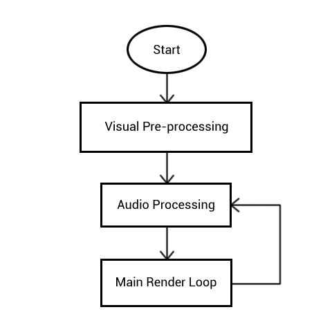
This is where I will discuss my actual implementation and how everything is structured! The following section will be broken down into three subsections that correspond to the actual order that things occur in:
The following is a flow diagram of how each step ensues. Notice the loop!
Visual Pre-processing
When procedurally generating visuals on the fly, it’s first a good idea to determine what elements are static and what are dynamic. By which I mean what elements need only be rendered once and re-used and what must be updated constantly. This separation is a good idea, as it means during the main render loop less computations have to be unnecessarily made. While developing the demo, there arose two situations where generating static content was necessary - the first was a displacement map, the second a spherical environment map. I’ll quickly explain what those are now!
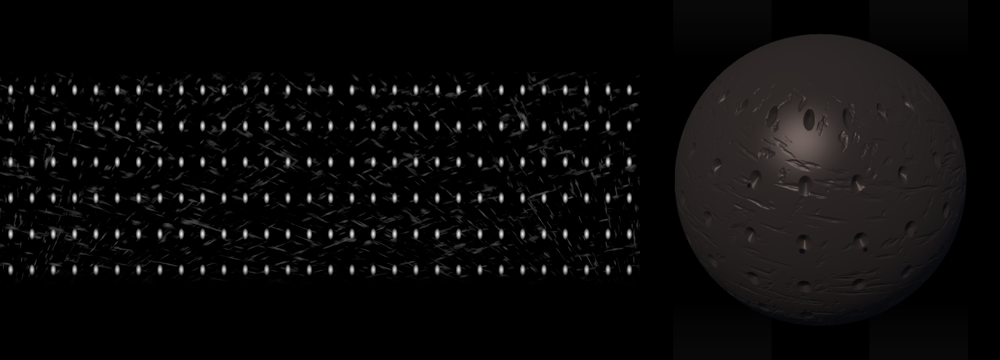
A displacement map is a specific kind of texture that encodes height values. In the following example, black pixels correspond to no change in height and white pixels refer to a maximum change in height. Grey values are a linear interpolation between the minimum and maximum.
I chose to use a displacement map over something like a normal map as one of the main advantages of signed distance fields is that they have infinite resolution. That is to say, the field is defined using a continuous distance value. Consequently, any infinitely precise point on the surface of the field can be described and therefore displaced. This is at an impasse with conventional polygonal representation, where the surface is determined by a discrete number of vertices. As this is the case, the surface can very easily be deformed with a displacement map using the ray marching technique while only taking the computational hit of a texture look up (and any further marches along the ray, but this is a given). Due to this, it makes sense to displace the geometry as it gives a much better result than bump mapping or normal mapping in that it produces an accurate silhouette.
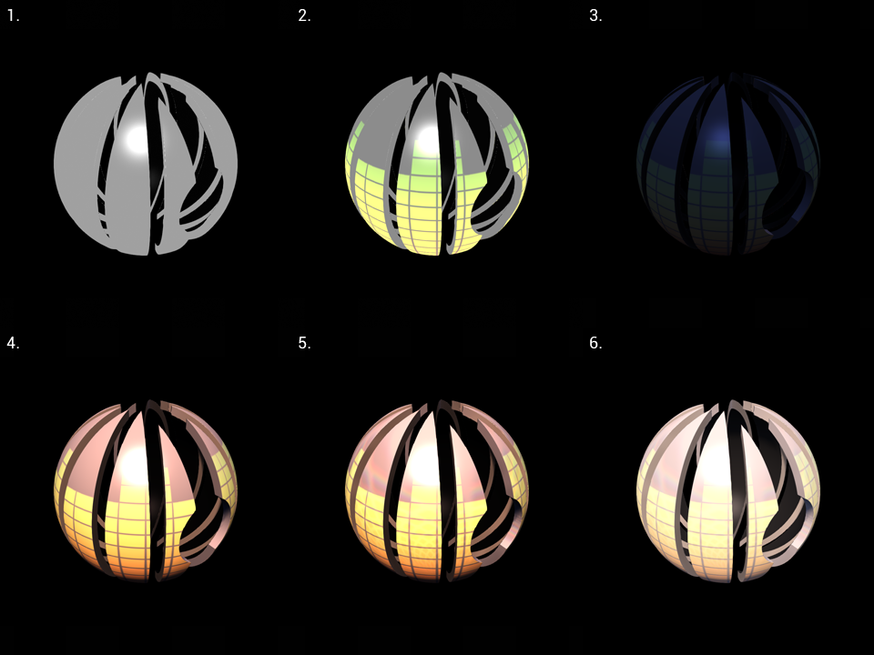
The other texture generated at this point is a spherical environment map used for the reflections in the outer shell of the object (seen below). This is a compromise - as I am using a ray marcher, ideally I would just march out another ray from the surface of the object along its normal vector to produce an accurate reflection. However, this is extremely costly, and unfortunately too costly for this demo to consistently run at an acceptable frame rate. Rendering this thing at 1080p was already super costly! Therefore I generated a spherical environment map; this is simply a texture similar to a panoramic photo that generates a full 360 degrees view of the room from the perspective of the object which can be sampled to produce the reflection. I opted to use a spherical environment map rather than, for instance, a cube map as the geometry is already a sphere and the poles of the sphere are not visible. This means that the “pinching” effect caused by the points of singularity at the poles of the sphere where the environment map converges aren’t visible.
Audio Processing
The next stage is actually inside of the main render loop, but concerns processing the audio as opposed to generating the visuals. The audio is the only part of the whole demo that is not procedurally generated (excluding the logo cough cough). The audio is stored in an MP3 file, then read in and analysed at runtime.
For the animations in the demo, frequency values are calculated from the audio on every iteration of the render loop. This is achieved using a Digital Signal Processing (DSP) technique called a Fast Fourier Transform (FFT). Anyone reading this that is familiar with audio processing probably already knows how FFTs work since they are very common! From a high level (since I am an audio noob), FFTs compute a Discrete Fourier Transform (DFT) where a signal is taken as input from, in this situation, a time domain and converts it into a value in the frequency domain. This means through this process, I can convert the audio stream signal into a series of frequency values where each value has a minimum of 0 and an undetermined maximum value. For the purposes of the animations however, I squished the values down so everything was between 0 and 1. For the demo, I calculated 256 frequency values and reduced this to a total of 4 frequency values.
Fortunately, I didn’t have to do these calculations myself. FMOD is a brilliant low-level library written in C++ that has DSP functionality. Rather than reinvent the wheel I made good use of FMOD instead! I’ll provide a link to the library at the bottom of the page, but feel free to ask about how I implemented FFTs in my demo as there aren’t a lot of resources online for the most up-to-date version of FMOD that describe how to do this.
Main Render Loop
We’re finally onto the main render loop! This is the crux of the whole demo, so it will have to be further broken down. Each sub-sub-section incorporates one render pass - this is where multipass rendering comes into play. A “pass” in this instance is where a fragment shader is executed for each pixel of the screen in parallel and rendered to a texture. Once the whole texture has been generated, it can then be passed into the next render pass to be sampled from (and rather importantly, this means neighbouring pixels on the texture can be sampled). Therefore, multipass rendering simply means multiple consecutive render passes to produce one final image.
There are four render passes in total:
Frequency Bars Pass
This first pass is used to generate the animated texture that can be seen mapped onto the surface of the shiny, white outer shell. Despite the next pass not requiring the sampling of neighbouring pixels, I split this into its own pass so it only had to be computed once per render loop. Rendering this was fairly trivial - hell, I’ll even give you the source code for this stage! The only slightly interesting part is that each bar uses an average of both the third and fourth frequency values, plus an additional pseudo-random value computed in the shader using a hash.
#version 430

//Texture coordinates (from vertex shader)
in vec2 vTexCoord;

//A tick value and the frequency values being passed in
uniform float tick;
uniform float levels[4];

//Hashing function, used to produce pseudo-random numbers
float hash(float n)
{
    return fract(sin(n) * 43758.5453123);
}

//Method for deciding on the colour (and height) of the bar
vec3 barColor(float y, float height, float currentLevel, float randomAddition)
{
  float additional = floor(hash(randomAddition * floor(tick * 4.0)) * 3.0);

  float bar = floor(y * height);
  vec3 color = mix(vec3(1.0, 0.0, 0.0), vec3(0.0, 1.0, 0.0), bar / height);
  color = clamp(currentLevel + additional, 0.0, bar) < bar ? vec3(0.0) : color;
  return clamp(color, 0.0, 1.0);
}

//Method for instancing the bars along the x-axis. Also performs some blending.
vec3 bars(vec2 uv, vec2 numberOfBars)
{
  vec3 color = barColor(uv.y, numberOfBars.y, floor((levels[2] + levels[3]) * 0.4 * numberOfBars.y), floor(uv.x * numberOfBars.x));

  vec2 fract_uv = fract(uv * numberOfBars);
  fract_uv = fract_uv * 2.0 - 1.0;
  vec2 amount = 1.0 - smoothstep(0.8, 1.0, abs(fract_uv));
  amount.y = amount.y * (1.0 - smoothstep(0.5, 1.0, sqrt(uv.y)));

  return color * min(amount.x, amount.y);
}

//Entry point
void main()
{
  gl_FragColor = vec4(bars(vTexCoord, vec2(40.0, 20.0)), 1.0);
}
Main Render Pass
Ok, this is the big one. In this stage, all of the aforementioned ray marching occurs, along with material computations for every object in the scene. Further to this, both direct and indirect shadows are calculated. There’s too much here to go into massive detail on each part, but I will of course include resources at the bottom of the page.
The first thing that happens in this stage is the initial scene setup. This includes defining where the camera is in the space and the direction that the ray for this pixel is moving in. Once these have been defined, ray marching can begin!
The ray marching stage is pretty much exactly as described previously. In this particular instance, the size of each step along the ray is determined by the estimated distance calculated at each step. This technique is good for detailed objects close to the camera but usually poor for something like terrain. For instances like terrain, I usually use fixed step sizes. To determine whether the ray has collided with an object, a global mapping function is used. The global mapping function simply contains all of the signed distance field definitions, along with an ID for each field that can be used to determine its material.
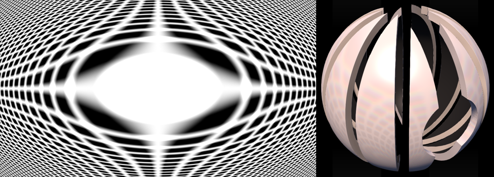
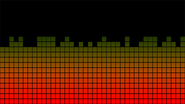
Once a collision occurs and an ID is returned, the material for the object must be calculated. This is entirely dependent on what object the ray collided with, so I will use the shiny, white outer shell as an example. The following is a series of screenshots showing how the material is built up. Please note that the actual calculations are for only one pixel at a time, but it’s more fun to show how the material looks at each stage as a whole! Another thing to note is that for the majority of the images, the colours are not gamma corrected, which makes the object look a little strange. Gamma correction is applied after the material has been created.
- 1. Firstly, the diffuse and specular colours are determined. This is what the material looks like "unlit".
- 2. Next, the bar texture computed in the previous pass is applied. The texture coordinates for the sphere are generated on the fly so that the texture can be warped to the surface of the sphere correctly.
- 3. Screen Space Ambient Occlusion is the next thing to be applied. This is a technique that estimates shadows produced by indirect lighting (i.e. the rays of light that bounce around and aren't absorbed by a material immediately). Note that the object looks quite blue at this point - this is because of the global illumination model I am using. There are three light sources in total; the "sun", the "sky" and an indirect light faking bounced rays from the "sun". Ambient occlusion is only calculated for the sky and and indirect light sources, and therefore the object ends up looking quite dark and blue. The techniques used to produce this lighting model can be found here.
- 4. Direct light and shadows are calculated at this point. Usually with ray marching, soft shadows are extremely computationally heavy to produce. However, by using signed distance fields, they can pretty much be calculated for free! A link to the technique used can be found here.
- 5. Finally, the reflections are applied to the material. This is where the environment map calculated in the visual pre-processing is used.
- 6. Once the material has been determined, gamma correction is applied. Gamma correction is a process that remaps the current colours of the scene into a linear space for computer monitors - I affectionately call this stage the "de-arsing" stage.
Motion Blur Pass
Once the main image is calculated, all that’s left to do is a couple of post-processing effects to improve the visuals. The main effect (separated into its own render pass) is motion blur. Typically with motion blur, you take a snapshot of the previous frame, compare it to the current frame and produce a vector field showing how much each pixel has moved. This can then be used to determine how much blurring needs to be applied to each pixel on the screen. However, to save on computation, I made the rather bold assumption that all moving pixels move at the same velocity.
Therefore all I have to do in this stage is compare the previous frame with the current frame, then blur the pixels that have changed by the speed that the camera is rotating at (determined by the frequencies calculated in the audio processing stage). This is technically not accurate, but can you reeeaaally tell?
I also applied a small amount of chromatic aberration at this stage just to add some colour to the motion blurring!
Post-processing Pass
The final pass just consists of a couple of small post-processing effects, such as anti-aliasing and the application of a noise filter and scanlines. Unfortunately, the noise filter and scanlines had to be removed for the video due to the effects producing artifacts with video compression… Trust me though, it looks dope in the actual application.
The anti-aliasing used is only FXAA. There is no particular reason for this besides it’s easy to apply, and adding the much better temporal anti-aliasing would take more time than I can be bothered to spend doing it. I will look into doing temporal anti-aliasing for my next demo!
That’s the whole rendering sequence complete!
Optimisation
One of the main problems with ray marching in real-time is that it can very quickly start affecting the frame rate. To counter this, various optimisations can be made. The main optimisations I used were the application of bounding volumes and Level of Detail (LOD) in the ambient occlusion and shadows.
Bounding volumes are basically simplified regions that encase more complex geometry. This means that before a position in space is compared to the complex geometry inside the volume, it is first compared to the volume itself. By doing so, only one calculation has to be made when outside the volume and the more complex geometry can be ignored until the position in space is actually inside the volume.
LOD is a pretty simply concept. For the ambient occlusion and shadows, the amount of detail (and therefore the amount of computations needed to calculate the effect) is determined by how far away the point in space is from the camera. Closer points require a higher amount of computations, whereas further away points require less. This is a very common technique and basically no clarity is lost from the image.
I also had to tweak the number of maximum steps the ray marcher could take when the camera zooms in. If you look closely at some of the concave areas of the object in the video when zoomed in, you can see weird black outlines and shapes - this is where the ray marcher reached its maximum steps before hitting the geometry! I willingly made this sacrifice to save on frames though. Note to self: use less concave and convex geometry next time!
Conclusions
I undertook this project over the period of a few weeks in my evenings. It’s not the first real-time ray marcher I’ve made, but it’s certainly the most complex. I aim to keep improving my skills and make better and better scenes in the future!
I have eluded to this person once previously in the post-mortem, but none of this would have been possible without the frankly incredible articles written by Íñigo Quílez. He is a co-creator of Shadertoy, prolific in Demoscene and has completed many articles, tutorials, lectures and talks in his time with computer graphics. I would highly recommend checking him out!
Shadertoy.com has also been an incredibly valuable resource for the procedural graphics programming, and 100% worth checking out if you’re interested in what I have been doing. It is a brilliant website for posting and viewing shaders, where the source code for every shader can be seen and modified in-browser through the power of WebGL. Word of warning though - if you haven’t got a competent GPU maybe stay away. You won’t be able to run any of the shaders very well, and it will definitely stall and crash your browser. ;)
That’s everything! Thank you for reading my post-mortem, and feel free to ask me any questions about specific parts!
Useful Links
Shadertoy.com - Basically the best website to learn shader programming on.
Examples of Ray Marching Signed Distance Fields by Íñigo Quílez - A bunch of demos produced by the man himself. They’re incredible, so check them out!
Articles by Íñigo Quílez - If you want to learn how to do effects like ambient occlusion, soft shadows, faked global lighting, etc. etc. then this is how I learned. The articles are full of typos, but they do a brilliant job of explaining all of the techniques I used in my demo.
Outdoor Lighting Model - This is a link to the outdoor lighting model that I used. There’s lots of useful stuff about setting up realistic looking lighting in this article.
Soft Shadows with Signed Distance Fields - It’s incredible easy to introduce soft shadows with Signed Distance Fields, so it’s definitely worth knowing!
FMOD - library used for DSP. There are plugins for Unity and Unreal, but if you’re like me and doing pure OpenGL you’ll want the low-level API download.
Unity Ray Marching Tutorial by Alan Zucconi - I didn’t use this personally, but I found it while researching for this post-mortem. It’s geared towards the Unity Engine though!
Ray marching Tutorial (In a Shader!) - I came across this on Twitter, but it’s super cool! It’s an interactive ray marching tutorial on Shadertoy. Would recommend!
Absolute Territory (MAJOR EPILEPSY WARNING) by Prismbeings